Pokémon Go! (démonstration Pandas/Seaborn)🔗
Voici un exemple d’utilisation des libraries Pandas (manipulation de données hétérogène) et Seaborn (visualisations statistiques), sur le Pokémon dataset d’Alberto Barradas.
Références:
[1]:
import pandas as PD
import seaborn as SNS
import matplotlib.pyplot as P

%matplotlib inline
Lecture et préparation des données🔗
Pandas fournit des méthodes de lecture des données à partir de nombreux formats, dont les données Comma Separated Values:
[2]:
df = PD.read_csv('./Pokemon.csv', index_col='Name')  # Indexation sur le nom (unique)
df.info()                                            # Informations générales
<class 'pandas.core.frame.DataFrame'>
Index: 800 entries, Bulbasaur to Volcanion
Data columns (total 12 columns):
#             800 non-null int64
Type 1        800 non-null object
Type 2        414 non-null object
Total         800 non-null int64
HP            800 non-null int64
Attack        800 non-null int64
Defense       800 non-null int64
Sp. Atk       800 non-null int64
Sp. Def       800 non-null int64
Speed         800 non-null int64
Generation    800 non-null int64
Legendary     800 non-null bool
dtypes: bool(1), int64(9), object(2)
memory usage: 75.8+ KB
Les premières lignes du DataFrame (tableau 2D) qui en résulte:
[3]:
df.head(10) # Les 10 premières lignes
[3]:
| # | Type 1 | Type 2 | Total | HP | Attack | Defense | Sp. Atk | Sp. Def | Speed | Generation | Legendary | |
|---|---|---|---|---|---|---|---|---|---|---|---|---|
| Name | ||||||||||||
| Bulbasaur | 1 | Grass | Poison | 318 | 45 | 49 | 49 | 65 | 65 | 45 | 1 | False |
| Ivysaur | 2 | Grass | Poison | 405 | 60 | 62 | 63 | 80 | 80 | 60 | 1 | False |
| Venusaur | 3 | Grass | Poison | 525 | 80 | 82 | 83 | 100 | 100 | 80 | 1 | False |
| VenusaurMega Venusaur | 3 | Grass | Poison | 625 | 80 | 100 | 123 | 122 | 120 | 80 | 1 | False |
| Charmander | 4 | Fire | NaN | 309 | 39 | 52 | 43 | 60 | 50 | 65 | 1 | False |
| Charmeleon | 5 | Fire | NaN | 405 | 58 | 64 | 58 | 80 | 65 | 80 | 1 | False |
| Charizard | 6 | Fire | Flying | 534 | 78 | 84 | 78 | 109 | 85 | 100 | 1 | False |
| CharizardMega Charizard X | 6 | Fire | Dragon | 634 | 78 | 130 | 111 | 130 | 85 | 100 | 1 | False |
| CharizardMega Charizard Y | 6 | Fire | Flying | 634 | 78 | 104 | 78 | 159 | 115 | 100 | 1 | False |
| Squirtle | 7 | Water | NaN | 314 | 44 | 48 | 65 | 50 | 64 | 43 | 1 | False |
Le format est ici simple:
nom du Pokémon (utilisé comme indice) et son n° (notons que le n° n’est pas unique)
type primaire et éventuellement secondaire str
différentes caractéristiques int (p.ex. points de vie, niveaux d’attage et défense, vitesse, génération)
type légendaire bool
Nous appliquons les filtres suivants directement sur le dataframe (inplace=True):
simplifier le nom des mega pokémons
remplacer les
NaNde la colonne «Type 2»éliminer les colonnes « # » et « Sp. »
[4]:
df.set_index(df.index.str.replace(".*(?=Mega)", ''), inplace=True)  # Supprime la chaîne avant Mega
df['Type 2'].fillna('', inplace=True)                               # Remplace NaN par ''
df.drop(['#'] + [ col for col in df.columns if col.startswith('Sp.')],
        axis=1, inplace=True)   # "Laisse tomber" les colonnes commençant par 'Sp.'
df.head()                       # Les 5 premières lignes
[4]:
| Type 1 | Type 2 | Total | HP | Attack | Defense | Speed | Generation | Legendary | |
|---|---|---|---|---|---|---|---|---|---|
| Name | |||||||||
| Bulbasaur | Grass | Poison | 318 | 45 | 49 | 49 | 45 | 1 | False |
| Ivysaur | Grass | Poison | 405 | 60 | 62 | 63 | 60 | 1 | False |
| Venusaur | Grass | Poison | 525 | 80 | 82 | 83 | 80 | 1 | False |
| Mega Venusaur | Grass | Poison | 625 | 80 | 100 | 123 | 80 | 1 | False |
| Charmander | Fire | 309 | 39 | 52 | 43 | 65 | 1 | False |
Accès aux données🔗
Pandas propose de multiples façons d’accéder aux données d’un DataFrame, ici:
via le nom (indexé):
[5]:
df.loc['Bulbasaur', ['Type 1', 'Type 2']] # Seulement 2 colonnes
[5]:
Type 1     Grass
Type 2    Poison
Name: Bulbasaur, dtype: object
par sa position dans la liste:
[6]:
df.iloc[-5:, :2] # Les 5 dernières lignes, et les 2 premières colonnes
[6]:
| Type 1 | Type 2 | |
|---|---|---|
| Name | ||
| Diancie | Rock | Fairy |
| Mega Diancie | Rock | Fairy |
| HoopaHoopa Confined | Psychic | Ghost |
| HoopaHoopa Unbound | Psychic | Dark |
| Volcanion | Fire | Water |
par une sélection booléenne, p.ex. tous les pokémons légendaires de type herbe:
[7]:
df[df['Legendary'] & (df['Type 1'] == 'Grass')]
[7]:
| Type 1 | Type 2 | Total | HP | Attack | Defense | Speed | Generation | Legendary | |
|---|---|---|---|---|---|---|---|---|---|
| Name | |||||||||
| ShayminLand Forme | Grass | 600 | 100 | 100 | 100 | 100 | 4 | True | |
| ShayminSky Forme | Grass | Flying | 600 | 100 | 103 | 75 | 127 | 4 | True |
| Virizion | Grass | Fighting | 580 | 91 | 90 | 72 | 108 | 5 | True |
Quelques statistiques🔗
[8]:
df[['Total', 'HP', 'Attack', 'Defense']].describe() # Description statistique des différentes colonnes
[8]:
| Total | HP | Attack | Defense | |
|---|---|---|---|---|
| count | 800.00000 | 800.000000 | 800.000000 | 800.000000 |
| mean | 435.10250 | 69.258750 | 79.001250 | 73.842500 |
| std | 119.96304 | 25.534669 | 32.457366 | 31.183501 |
| min | 180.00000 | 1.000000 | 5.000000 | 5.000000 |
| 25% | 330.00000 | 50.000000 | 55.000000 | 50.000000 |
| 50% | 450.00000 | 65.000000 | 75.000000 | 70.000000 |
| 75% | 515.00000 | 80.000000 | 100.000000 | 90.000000 |
| max | 780.00000 | 255.000000 | 190.000000 | 230.000000 |
[9]:
df.loc[df['HP'].idxmax()] # Pokémon ayant le plus de points de vie
[9]:
Type 1        Normal
Type 2
Total            540
HP               255
Attack            10
Defense           10
Speed             55
Generation         2
Legendary      False
Name: Blissey, dtype: object
[10]:
df.sort_values('Speed', ascending=False).head(3) # Les 3 pokémons plus rapides
[10]:
| Type 1 | Type 2 | Total | HP | Attack | Defense | Speed | Generation | Legendary | |
|---|---|---|---|---|---|---|---|---|---|
| Name | |||||||||
| DeoxysSpeed Forme | Psychic | 600 | 50 | 95 | 90 | 180 | 3 | True | |
| Ninjask | Bug | Flying | 456 | 61 | 90 | 45 | 160 | 3 | False |
| DeoxysNormal Forme | Psychic | 600 | 50 | 150 | 50 | 150 | 3 | True |
Statistiques selon le statut « légendaire »:
[11]:
legendary = df.groupby('Legendary')
legendary.size()
[11]:
Legendary
False    735
True      65
dtype: int64
[12]:
legendary['Total', 'HP', 'Attack', 'Defense', 'Speed'].mean()
[12]:
| Total | HP | Attack | Defense | Speed | |
|---|---|---|---|---|---|
| Legendary | |||||
| False | 417.213605 | 67.182313 | 75.669388 | 71.559184 | 65.455782 |
| True | 637.384615 | 92.738462 | 116.676923 | 99.661538 | 100.184615 |
Visualisation🔗
Pandas intègre de nombreuses fonctions de visualisation interfacées à matplotlib.
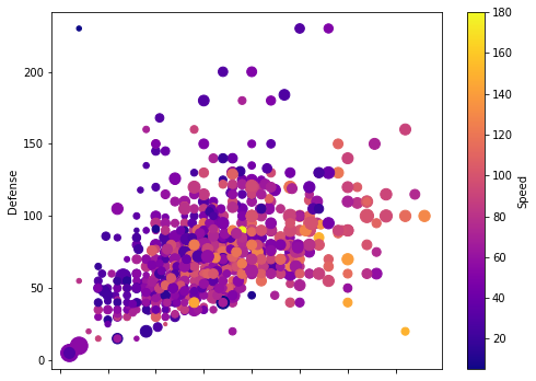
[13]:
ax = df.plot.scatter(x='Attack', y='Defense', s=df['HP'], c='Speed', cmap='plasma')
ax.figure.set_size_inches((8, 6))
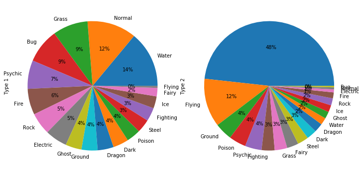
[14]:
fig, (ax1, ax2) = P.subplots(1, 2, subplot_kw={"aspect": 'equal'}, figsize=(10, 6))

df['Type 1'].value_counts().plot.pie(ax=ax1, autopct='%.0f%%')
df['Type 2'].value_counts().plot.pie(ax=ax2, autopct='%.0f%%')

fig.tight_layout()
Il est également possible d’utiliser la librairie seaborn, qui s’interface naturellement avec Pandas.
[15]:
pok_type_colors = {    # http://bulbapedia.bulbagarden.net/wiki/Category:Type_color_templates
  'Grass': '#78C850',
  'Fire': '#F08030',
  'Water': '#6890F0',
  'Bug': '#A8B820',
  'Normal': '#A8A878',
  'Poison': '#A040A0',
  'Electric': '#F8D030',
  'Ground': '#E0C068',
  'Fairy': '#EE99AC',
  'Fighting': '#C03028',
  'Psychic': '#F85888',
  'Rock': '#B8A038',
  'Ghost': '#705898',
  'Ice': '#98D8D8',
  'Dragon': '#7038F8',
  'Dark': '#705848',
  'Steel': '#B8B8D0',
  'Flying': '#A890F0',
}
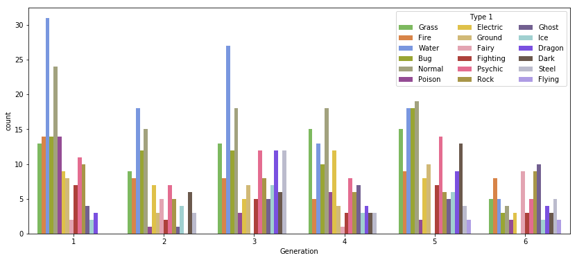
[16]:
ax = SNS.countplot(x='Generation', hue='Type 1', palette=pok_type_colors, data=df)
ax.figure.set_size_inches((14, 6))
ax.legend(ncol=3, title='Type 1');
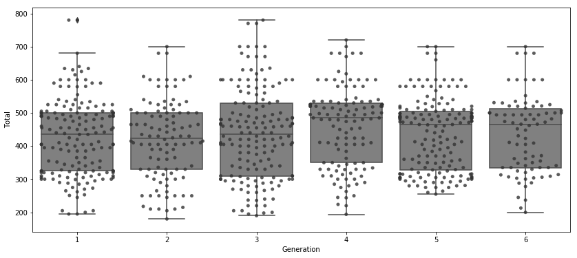
[17]:
ax = SNS.boxplot(x='Generation', y='Total', data=df, color='0.5');
SNS.swarmplot(x='Generation', y='Total', data=df, color='0.2', alpha=0.8)
ax.figure.set_size_inches((14, 6))
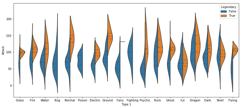
[18]:
ax = SNS.violinplot(x="Type 1", y="Attack", data=df, hue="Legendary", split=True, inner='quart')
ax.figure.set_size_inches((14, 6))
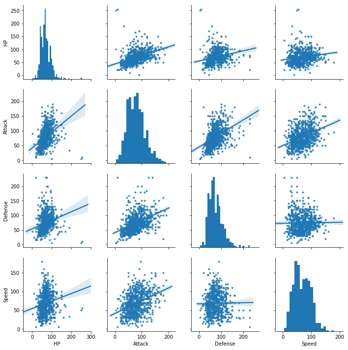
[19]:
df2 = df.drop(['Total', 'Generation', 'Legendary'], axis=1)
SNS.pairplot(df2, markers='.', kind='reg');
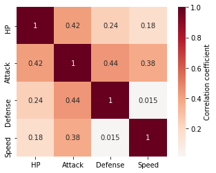
[20]:
ax = SNS.heatmap(df2.corr(), annot=True,
                 cmap='RdBu_r', center=0, cbar_kws={'label': 'Correlation coefficient'})
ax.set_aspect('equal')
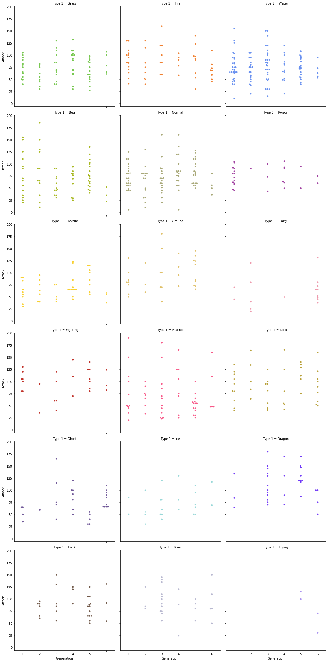
[21]:
SNS.catplot(x='Generation', y='Attack', data=df,
               hue='Type 1', palette=pok_type_colors, col='Type 1', col_wrap=3, kind='swarm');
This page was generated from Cours/pokemon.ipynb.